BXL cobblestones

Inspired by the many beautiful prints of city road networks (see for example Andrei Kashcha's beautiful city roads website), I wanted to make one for Brussels myself. In R! By chance, I found a dataset of all the cobblestone streets in Brussels, which I thought would be a nice little addition to a map of Brussels. And besides Brussels = Belgium = cycling = cobblestones!

I found the cobblestone data on the Brussels Open Data Store and downloaded it in geojson format, thinking that would be the easiest to plot in R (small disclaimer: I have little experience with cartography and plotting maps, so the way I did things is probably, maybe not the most efficient). As always, you can find the geojson data and R code on GitHub.

Now where could I find the road network data for Brussels? After some digging around in the GitHub repo for the city roads website, I learned that it downloaded the data from OpenStreetMap using Overpass API queries (basically an API that serves custom selected parts of the OSM map data). That's a lot of stuff I'm not familiar with! Luckily, and unsurprisingly I should say, there's an R library for that. Let's get started!

					
library('osmdata')
library('tidyverse')
library('sf')
library('geojsonio')
library('rgdal')

# Delimit the area we're going to plot. The idea is to have the Brussels
# "pentagon" (the city center surrounded by the small ring road) roughly
# in the center of the poster. I picked the delimiting latitude and
# longitude values by hand.
boundingBox = matrix(c(4.3, 4.4, 50.8, 50.9), nrow=2, ncol=2, byrow=TRUE)
colnames(boundingBox) = c('min', 'max')
rownames(boundingBox) = c('x', 'y')

# Get a map with all the roads (which, for some reason, are called
# highways) in Brussels from OpenStreetMap using an Overpass query.
streets = opq(boundingBox) %>%
		  add_osm_feature('highway') %>%
		  osmdata_sf()
allStreetsGeom = streets$osm_lines$geometry

# Load the cobblestone dataset. I downloaded these data from the
# Brussels Open Data Store:
# http://opendatastore.brussels/dataset/paved-roads
cobbles = geojson_read('cobblestonesBrussels.json', what='sp')
					
				

Alright! I have all the data I need, only thing left to do is to plot them. If only it was that easy... Plotting either the OSM road network or the cobblestone streets was pretty easy, but I just could not get them together in a single figure. Instead, I basically loop through the different geometries (the roads and cobblestone streets) and draw them using their coordinates and the base plot function. I'm sure there is an easier or more straightforward way to do this, but hey, it works!

All done, right? Unfortunately not. Once I managed to get all the data together in one plot, it was immediately obvious that the OSM and cobblestone streets did not overlap. Which I assumed they would, because why not? Cue some more frustrated googling/DuckDuckGo-ing. And this is where I learned about the existence of a seemingly endless number of different coordinate systems. Apparently, OSM uses the so-called EPSG:4326 coordinate system ^[1], which is easy enough to find online. Figuring out the coordinate system used for the cobblestone streets was unfortunately not straightforward. After I found epsg.io/transform, an online coordinate system transformation tool, I manually tried out different systems to see which one lined up with the OSM coordinates after being converted to EPSG:4326. Luckily, I noticed that there are country-specific coordinate systems, so I tried searching for Belgian coordinate systems and that ended up saving me a lot of time.

					
pdf('cobblestones_brussels.pdf', width=11.69, height=16.53)
par(bg=NA, mar=c(2, 2, 2, 2))
plot(0, 0, type='n', xlim=boundingBox['x',], ylim=boundingBox['y',], xlab='', ylab='', bty='n', xaxt='n', yaxt='n')
for (i in 1:length(allStreetsGeom)) {
	lines(st_coordinates(allStreetsGeom[i]), lwd=0.5, col='#abacb0')
}
for (i in 1:length(cobbles)) {
	cblCoor = cobbles@polygons[[i]]@Polygons[[1]]@coords %>%
			  data.frame()
	colnames(cblCoor) = c('lon', 'lat')
	coordinates(cblCoor) = c('lon', 'lat')
	proj4string(cblCoor) = CRS('+init=epsg:31370')
	cblCoorNew = spTransform(cblCoor, CRS('+init=epsg:4326'))
	lines(cblCoorNew@coords, lwd=1, col='#393e46')
}
dev.off()
					
				

While this project turned out to be a little bit more complex than I had initially imagined, I'm quite pleased with the result! I added a small legend and my name to the map using Illustrator, but other than that, everything was done in R. Let me know what you think @monsieurKoch! Any tips on how to simplify the plotting would also be greatly appreciated :)

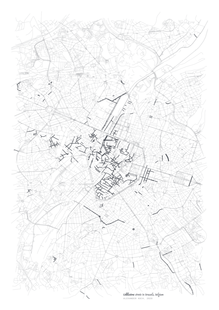
You can find the high-res version of this map on GitHub: cobblestones_brussels.pdf